Tutorial C2 - Reconstruction of shape parameter and optical constants

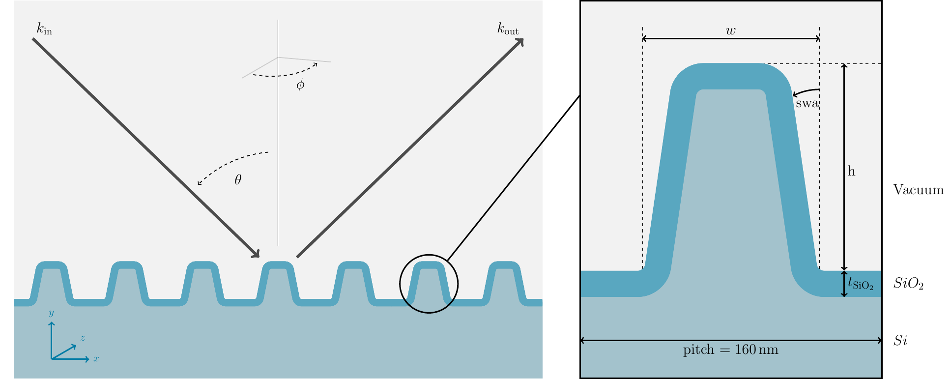
In this example we want to show how we want use a forward simulation of a scatterometry measurement for the reconstruction of shape parameter of the sample and the optical constants of the materials by using an Markov Chain Monte Carlo arlgorithm (MCMC). In scatterometry a light beam of a certain energy is scatterd at the sample and reflected on a detector. For this example we simulated the scatterometry measurement of a periodic line-grating with a pitch of \(160\,\mathrm{nm}\). The grating consists of a silicone bulk with a native oxide-layer on top and is defined by several geometric parameters as it is shown in the image below togehter with details about the measurement.

Measurement setup:

energies \(\boldsymbol{95.4}\) eV, \(105.0\) eV, \(109.9\) eV
s-polarization
incidence angle \(\theta = 60^\circ\)
azimuthal angle \(\phi \in [90^\circ, 96^\circ]\)

Forward simulation

For the simulation of the measurement we used a finite element solver from JCMsuite (https://www.docs.jcmwave.com/JCMsuite/html/index.html) and made the measurement simulations for three different energies. In the present example we will just use the first one. The shape of the line-grating is defined by the geometric parameters heigth, width, side-wall-angle, thickness of oxide layer, and the behavoir of the material by the optical constants for silicon (\(\mathrm{Si}\)) and silicon-oxide (\(\mathrm{Si0}_2\)), wich are given as a function of the material densities \(\rho_{\mathrm{SiO}_2}\) and \(\rho_{\mathrm{Si}}\) using the information from databases. For \(\mathrm{SiO}_2\) the information comes from OCDB (https://www.ocdb.ptb.de/home) from the PTB and for \(\mathrm{Si}\) the values were taken from CXRO-Database (https://henke.lbl.gov/optical_constants/getdb2.html). To describe the line-edge roughness we used the Deby-Waller factor depending on an aditional parameter \(\sigma_\mathrm{roughnes}\). The corner roundings of the grating lines are set to the fix value of \(5\,\mathrm{nm}\) at the top and \(10\,\mathrm{nm}\) at the bottom. Hence the forward model depends on \(7\) parameters

\[x=(\mathit{h},\mathit{w},\mathit{swa}, \mathit{th}_{\mathit{SiO}_2}, \rho_{\mathit{SiO}_2}, \rho_{\mathrm{Si}}, \sigma_{\mathrm{rough}})\]

and determines for the \(x\)-parameter the intensities of the diffraction orders from \(-5\) to \(5\), hence for one parameterset \(x\) the forward evaluation \(f(x)\) has the shape \((7,11)\).

Inverse Problem

The aim is to solve the inverse problem, that means we want to determine the unknwon parameter contained in \(x\). Therefore we use Bayesian Inversion in the following way. The measurement data \(y\) is described by the forward model \(f\) plus the model error \(\varepsilon\) and the measurement noise \(\eta\) which are both given as random variables. The model error comes from inaccuracies of the forward model and the measurement noise is caused by deviations of the measuring instrument. We assume here, that both random variables are Gaussian distributed such that the measurement data \(y\) is given by

\[y = f(x) + \varepsilon + \eta \qquad \text{for}\]

\(f(x)\) – forward model of \(x\)
\(\varepsilon \sim \mathcal{N}(0, \Sigma_{\varepsilon})\) – model error
\(\eta \sim \mathcal{N}(0, \Sigma_{\eta})\) – measurement noise

The distribtions for model error and noise are defined in detail below in the section about the error model.

import time
import numpy as np
import pythia as pt
import matplotlib.pyplot as plt
import pandas as pd
import emcee
from _src.prob_functions import log_likelihood, log_prior_uniform
from _src.eval_reconstruction import corner_plot

Surrogate Model

Since the MCMC algorithm needs to evaluate the forward model many times we are going to use a surrogate model that is faster to evalute. To this we approximate the forward model by a polynomial chaos expansion (PCE) using the python packague PyThia. Therefore we define for each parameter a domain and a distribution. Below you can see the parameter information used in this example.

Shape and material parameter definitions with their respective domains and distributions.
#	Parameter	Distribution	Domain
1	height_line	uniform	\([120.0, 140.0]\)
2	width_line	uniform	\([80.0, 100.0]\)
3	thick_sio2	uniform	\([1.5, 2.5]\)
4	swa	uniform	\([0.0, 5.0]\)
5	rho_sio2	uniform	\([0.0, 6.0]\)
6	rho_si	uniform	\([0.0, 6.0]\)
7	sigma_roughness	uniform	\([0.0, 2.0]\)

To define the parameters in python we can use the following code.

param1 = pt.parameter.Parameter(name="height_line", domain=[120., 140.], distribution="uniform")
param2 = pt.parameter.Parameter(name="width_line", domain=[80., 100.], distribution="uniform")
param3 = pt.parameter.Parameter(name="thick_sio2", domain=[1.5, 2.5], distribution="uniform")
param4 = pt.parameter.Parameter(name="swa", domain=[0., 5.], distribution="uniform")
param5 = pt.parameter.Parameter(name="rho_sio2", domain=[0., 6.], distribution="uniform")
param6 = pt.parameter.Parameter(name="rho_si", domain=[0., 6.], distribution="uniform")
param7 = pt.parameter.Parameter(name="sigma_roughness", domain=[0., 2.], distribution="uniform")
params = [param1, param2, param3, param4, param5, param6, param7]

Next we have to choose which polynomial degrees we want to include in the surrogate model. Here we define the index set of the corresponding multiindices using pt.index.lq_bound_set(dimensions, b, q). Hence all indices with an \(l_q\)-Norm smaller or equal than a bound b are choosen for the approximation.

indices_lq_bound = pt.index.lq_bound_set(np.ones(nmb_params) * 12, bound=12, q=0.5)
index_set = pt.index.IndexSet(indices_lq_bound)

The multiindex information below show details about PC-approximation.

Multiiindex information.
Key	Value
number of indices	\(575\)
dimension	\(7\)
maximum dimension	\([11, 11, 11, 11, 11, 11, 11]\)
number of sobol indices	\(127\)

To define the PCE we use forward evaluations on the parameter domain

\[\Omega= [a_1, b_1]\times \ldots \times [a_7, b_7]\]

from the original forward model. Therefore we load nearly \(10.000\) samples and the corresponding evaluations. The samples are then divided in a training set and a test set. The training set will be used to define the PCE and the test set to check the approximation error.

# load data
energy = 95.4
path_samples = "../../_data/samples_and_feval/samples_eval_setup2/"
samples_load = np.load(path_samples + "valid_samples_uniform" + "_lg_c2_2_density" + ".npy")
fx_load = np.load(path_samples + f"intensity_lg_c2_2_density_{energy}eV.npy")

fx = fx_load[:, :, 0]
for ii in range(1, fx_load.shape[-1]):
    fx = np.concatenate((fx, fx_load[:, :, ii]), axis=-1)

# training samples
N_train = 9000
samples_train = samples_load[:N_train]
fx_train = fx[:N_train]
weights_train = 1 / N_train * np.ones(samples_train.shape[0])

# test set to check the approximation error
samples_test = samples_load[N_train:]
fx_test = fx[N_train:]
nmb_test_samples = samples_test.shape[0]

With this setting, we have \(9000\) training and \(894\) test data samples. Next, we need to compute the polynomial chaos surrogate using PyThia. Fortunately, this is only one simple command which takes roughly \(19\,\mathrm{s}\) to compute a surrogate.

pce = pt.chaos.PolynomialChaos(
   params,
   index_set,
   x_train=samples_train,
   w_train=weights_train,
   y_train=fx_train
)

Approximation Error

The approximation error of the surragate model is calculated on a test set of samples. Here we first take for each component of the functions the average over the test set of samples \(\{x_i\}_{i=1}^N\) given by

\[\Vert g_k \Vert_{L_2}^2 = \frac{1}{N} \sum_{i=1}^N \vert g_k(x_i) \vert^2\]

and then we average over all components to get the \(L_2\) error for the whole function. The here used errors are an absolute and relative \(L_2\) error given by

absolute \(L_2\) error: \(\frac{1}{K} \sum_{k = 1}^K \Vert f_k - \tilde{f}_k \Vert_{L_2}^2\)
relative \(L_2\) error: \(\frac{1}{K} \sum_{k = 1}^K \frac{\Vert f_k - \tilde{f}_k \Vert_{L_2}^2}{\Vert f_k \Vert_{L_2}^2}\).

To compute the approximation errors, we can use the following lines of code.

pce_test = pce.eval(x=samples_test)
dim_img = pce_test.shape[-1]

L2_norm_fx = np.sum(fx_test**2, axis=0) / nmb_test_samples
L2_norm_diff = np.sum((pce_test - fx_test) ** 2, axis=0) / nmb_test_samples

abs_L2_error = np.sqrt(np.sum(L2_norm_diff, axis=-1) / dim_img)
rel_L2_error = np.sqrt(np.sum((L2_norm_diff / L2_norm_fx), axis=-1) / dim_img)

In our case, the absolute and relative \(L_2\) errors end up to be \(1.04\cdot 10^{-4}\) and \(0.18\), respectively.

Error Model

We have to define an error model, describing the mode error \(\varepsilon\) and measurement nosie \(\eta\). Here we assume, that both random variables are Gaussian distributed

\(\varepsilon \sim \mathcal{N}(0, \Sigma_{\varepsilon})\) – model error
\(\eta \sim \mathcal{N}(0, \Sigma_{\eta})\) – measurement noise

With the variances given by:

Model Error: \(\Sigma_{\varepsilon} = \operatorname{diag}(\sigma_{1,\varepsilon}^2, \ldots ,\sigma_{1,\varepsilon}^2 )\) for \(~\sigma_{j,\varepsilon}^2 = (a \cdot y_j)^2 + b^2\)
Measurement Nosie: \(\Sigma_{\eta} = \operatorname{diag}(\sigma_{1,\eta}^2, \ldots ,\sigma_{1,\eta}^2 )~\) for \(~\sigma_{j,\eta}^2 =( c \cdot y_j )^2\)

Since the measurement noise can be determined quite precisely it was set to a certain percentage of the measurement. The model error depends on two hyperparameters \(a,b\), which are going to be determined within the reconstruction of the model parameter. The main idea is to describe a background noise of the measurement by the parameter \(b\) and a fluctuation of the lightbeam by \(a\). To setup the error model we use the following lines of code.

# add hyperparameter for model error
a = 0.01
b = 1e-5
c = 0.01

param_a = pt.parameter.Parameter(name="me_a", domain=[0, 0.3], distribution="uniform")
param_b = pt.parameter.Parameter(name="me_b", domain=[0, 1e-4], distribution="uniform")
hyper_params = [param_a, param_b]

nmb_hyper_params = len(hyper_params)
domains = [p.domain for p in params + hyper_params]
param_names = [p.name for p in params + hyper_params]

MCMC Reconstruction

For the reconstruction we use an MCMC algorithm, wich generates independent samples from the posterior distribution of the parameter contained in \(x\). In this example we use synthetic data generated by the forward model. The measurement is then replaced by the synthetic data defined as

\[y^{\star} = f(x^{\star}) + \varepsilon^{\star} + \eta^{\star}\]

for a random drawn sample \(x^{\star} =\) x_true \(\sim\mathcal{U}(\Omega)\) for the parameter domain \(\Omega\) and samples for noise and model error \(\varepsilon^{\star}\) and \(\eta^{\star}\) drawn from \(\mathcal{N}(0, \Sigma_{\varepsilon})\) and \(\mathcal{N}(0, \Sigma_{\eta})\) respectively.

prior = pt.sampler.ParameterSampler(params + hyper_params)
x_true = prior.sample(1)[0]
x_true[-nmb_hyper_params:] = np.array([a,b])

fx_true = pce.eval(x=x_true[:-nmb_hyper_params])
sigma_me_sq = (a * fx_true) ** 2 + b**2
sigma_noise_sq = (c * fx_true) ** 2
sigma = np.sqrt(sigma_me_sq + sigma_noise_sq)
model_error = np.random.normal(0, sigma)

syn_data = fx_true + model_error

To use an MCMC sampler from the python packague emcee (https://github.com/dfm/emcee) we define a forward model function and a log-posterior function, which gets as only input the parameter, respectively parameter + hyperparameter. The log-posterior is given by

\[\ell(x;y) = -\frac{1}{2} (y-f(x))\cdot\Sigma^{-1}(y-f(x)).\]

for \(\Sigma = \Sigma_{\varepsilon} + \Sigma_{\eta}\).

def log_posterior(x):
    params_x = x[:-nmb_hyper_params]
    a_me = x[-nmb_hyper_params]
    if b != 0:
        b_me = x[-1]
    else:
        b_me = b
    c_noise = c

    log_likeli = log_likelihood(
        y=syn_data, x=params_x, f=pce_surrogate.eval(x), a=a_me, b=b_me, c=c_noise
    )
    log_prior = log_prior_uniform(x=x, dom=domains)
    log_post = log_likeli + log_prior
    return log_post, log_prior

MCMC setup

To start the MCMC algorithm we need to define a number of chains we want to start and the chain-lenght, meaning the number of samples that are drawn in each chain. The chains are initialized by a random sample from the parameter domain using prior.sample(N_CHAINS). Then the sampler is defined, containg as input parameter the dimensions (number of chains, number of parameter) and the log-posterior. Then the sampler can be started.

N_CHAINS = 20
CHAIN_LENGTH = 5000
FILENAME = "mcmc_backup"
BACKUP_INTERVAL = 100
BURN_IN = 200
p0 = prior.sample(N_CHAINS)
ndim = len(domains)

index = 0
autocorr = np.empty(CHAIN_LENGTH)
act_x, act_t = [], []

First we make an MCMC run only for a small number of samples, in order to get to a point which is independent from the initialisation of the chains. This is called the burn-in. Then the real mcmc run is started.

sampler = emcee.EnsembleSampler(N_CHAINS, ndim, log_posterior)
state = sampler.run_mcmc(p0, BURN_IN, progress=True)
sampler.reset()

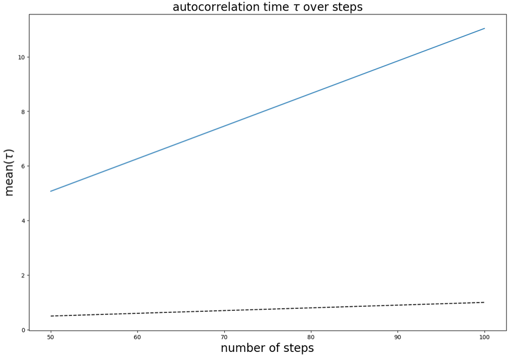
During the run the autocorrelation-time and acception fraction are saved at regular intervals (backup-interval) for monitoring and check of convergence criteria. As convergence criteria we use the autocorrelation lenght and the Gelamn-Rubin criteria, which are shown below.

for sample in sampler.sample(state, iterations=CHAIN_LENGTH, progress=True):

    if sampler.iteration % BACKUP_INTERVAL:
        continue

    tau = sampler.get_autocorr_time(tol=0)
    autocorr[index] = np.mean(tau)
    index += 1
    act_x.append(sampler.iteration)
    act_t.append(np.mean(tau))
    accept_frac = sampler.acceptance_fraction

Monitoring

After the MCMC run is finished we check the autocorrelation time. Since we only want to have independent samples we define a thin value, that describes how many samples we have to skip in order to get an independent sample. We also define again a burn-in depending on the autocorrelation time. For the posterior samples we only use samples from the thinned chains after the burn-in. Below you can see these values as well as convergence criteria as the autocorrelation time, acceptance rate and gelman-rubin. We assume the algorithm to be converged, if gelman-rubin is close to :math`1` and the autocorrelation time times \(100\) is smaller than the number of iterations.

# saving and monitoring
act = sampler.get_autocorr_time(tol=0)
burnin = int(2 * np.max(act))
thin = int(0.5 * np.min(act))

# select only samples each thin step
post_samples = sampler.get_chain(discard=burnin, flat=True, thin=thin)
samples_chains = np.swapaxes(sampler.get_chain(flat=False), 0, 1)

Example MCMC monitoring values and convergence criteria.
Monitoring Parameter	Value
time	\(4\, \mathrm{min}\ 15\,\mathrm{s}\)
number of samples	\(360\)
burn-in	\(25\)
thin	\(4\)
mean ac time	\(11.035535269258625\)
mean acpt. rate	\(0.22049999999999997\)
mean gelman-rubin	\(1.8790655719638443\)

This condition can be checked in the autocorrelation-plot below. The autocorrelation value has to cross the dashed line.

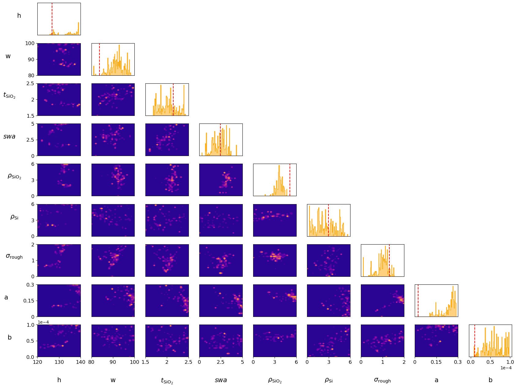
Posterior distribution

The selected samples are now distributed after the posterior distribution. In the corner plot below, you can see the distribution for each parameter on the diagonal and for each parameter combination of two parameter. The mean values, variances and confidence intervals are shown below.

means = np.mean(post_samples, axis =0)
variances = np.var(post_samples, axis=0)
conf_interval = list(pt.misc.confidence_interval(post_samples))

Ground truth, reconstruction values and associated uncertainties.
#	parameter	domain	true value	mean	variance	conf. interval
1	\(\mathit{h}\)	\([120,140]\)	\(126.24\)	\(134.24\)	\(26.8\)	\([125.8,139.9]\)
2	\(\mathit{w}\)	\([80,100]\)	\(83.09\)	\(91.93\)	\(14.7\)	\([84.0,98.3]\)
3	\(\mathit{th}_{\mathrm{SiO}_2}\)	\([1.5,2.5]\)	\(2.16\)	\(2.02\)	\(0.1\)	\([1.7,2.4]\)
4	\(\mathit{swa}\)	\([0,5]\)	\(2.45\)	\(2.30\)	\(0.8\)	\([0.5,3.8]\)
5	\(\rho_{\mathrm{SiO}_2}\)	\([0,6]\)	\(5.34\)	\(3.71\)	\(0.3\)	\([2.7,4.5]\)
6	\(\rho_{\mathrm{Si}}\)	\([0,6]\)	\(2.96\)	\(2.40\)	\(2.3\)	\([0.1,5.2]\)
7	\(\sigma_r\)	\([0,2]\)	\(1.34\)	\(0.97\)	\(0.1\)	\([0.0,1.5]\)
8	\(a\)	\([0,3]\)	\(0.01\)	\(0.24\)	\(2.8\cdot10^{-3}\)	\([0.1,0.3]\)
9	\(b\)	\([0,10^{-4}]\)	\(10^{-5}\)	\(5.9\cdot10^{-5}\)	\(5.5\cdot10^{-10}\)	\([0.0, 9.7\cdot10^{-5}]\)