Tutorial C1 & C3 - Reconstruction of optical constants of thin layer systems using MCMC

This tutorial will guide you through the necessary steps in reconstructing the geometric parameters as well as the optical contants (OC) of a thin layer system using Markov chain Monte Carlo (MCMC). We will use data obtained by EUV reflectometry by PTB work group 7.14 as a basis for the reconstruction process.

The reconstruction will yield samples from the posterior distributions of the

geometric parameters - thickness \(d\) - roughnesses \(\sigma_1\), \(\sigma_2\)
optical constants \(n( \lambda)\) and \(k( \lambda)\)
error model parameters \(a,b\)

The error model \(y=af(x)+b\) tries to estimate the uncertainties introduced by our employed forward model and the numerical handling of the problem. Forward modeling is done via the Transfer Matrix Method (https://doi.org/10.1364/AO.447152) and maps the input parameters to the reflectance data.

Preprocessing and running the reconstruction

The required Python packages are indicated in an requirements.txt (for ussage with pip) which is available together with the required source code in the ATMOC Gitlab repository (https://gitlab1.ptb.de/ptb-843/atmoc-oc-reconstruction-tutorial).

We will use a simple two Layer model for recontructing the OC of a \(30\,\mathrm{nm}\) Ruthenium sample on top of a Silicon bulk substrate. Configuration of the parameters is handled within two files multilayer_setups.py and parameters.py.

The configuration for the layer system is handled in multilayer_setups.py and we will use the setup shown below. The MCMC procedure requires an input of prior distributions. These are chosen to be uniform distributions \(\mathcal{U}(\mathit{lb},\mathit{ub})\) and a reasonable choice for the lower bound \(\mathit{lb}\) as well as the upper bound \(\mathit{ub}\) has to be given for every parameter to be reconstructed.

For the geometric and error model parameters, these bounds are defined in multilayer_setups.py, while the prior bounds for the OC are derived from pre-calculated theoretical estimates in combination with a choosable range, defined in parameters.py.

## Ru 30 nm single layer

# Local Path to store the results and automated postprocessing
prefix = "./"

Ru_30nm_1_layer_00 = mcmc_setup(
    layers=["Ru"],
    thickness=np.asanyarray([30]),
    mat="Ru",
    errortype="abs",
    error_params=np.asanyarray([0.01, 1e-5]),
    # Bounds (Uppper/Lower bound) for the error model parameters [a,b]
    error_bounds=np.asanyarray([[0.25, 1e-6 + 5 * 1e-7], [0.0005, 1e-6 - 5 * 1e-7]]),
    roughness=np.asanyarray([1, 1]),
    # error bounds for the geometric parameters
    # [thickness, roughness top, roughness layer/substrate]
    geo_bounds=np.asanyarray([[33, 1.25, 1.25], [27, 0.75, 0.75]]),
    measured_thickness=30,
    # s-polarisation
    polarization=1,
    oc_bound_type="abs",
)
setups = [Ru_30nm_1_layer_00]

An extension to this model to include an oxidation layer is also included in the tutorials/ folder.

To summarise the chosen model parameters and parameter bounds:

Material and hyper parameters with their respective domain bounds.
#	parameter	upper bound	lower bound
1	thickness \(d\)	\(33\,\mathrm{nm}\)	\(27\,\mathrm{nm}\)
2	roughness \(\sigma_1\)	\(1.25\,\mathrm{nm}\)	\(0.75\,\mathrm{nm}\)
3	roughness \(\sigma_2\)	\(1.25\,\mathrm{nm}\)	\(0.75\,\mathrm{nm}\)
4	error parameter \(a\)	\(0.25\)	\(5 \cdot 10^{-4}\)
5	error parameter \(b\)	\(15 \cdot 10^{-7}\)	\(5 \cdot 10^{-7}\)

The second configuration file parameter.py handles the parameters for the MCMC procedure as well as the location of the precalculated material parameters, if present. In our case, these are the optical constant estimates for Ru as well as the theoretical values for the Si bulk material. Note that the OC of the bulk substrate material are not reconstructed and therefore fixed. The variables deltabound and betabound set the upper and lower boundaries for the OC priors for the real and imaginary part of the OC, adding or substracting the given factor from the theoretical estimates.

mcmc_poolsize = 8  # Number of CPUs to be used
nsteps_mcmc = 3  # 100000 MCMC steps in emcee
step_interval = 1000  # interval after which convergence is checked
thin = 10  # Thin the drawn samples by this factor
walker_multiplier = 1024  # How many independent walkers to launch for each parameter
burnin_factor = 6.0
burnin = nsteps_mcmc / burnin_factor

materials = {
    "Vacuum": {},
    "Si": {
        "oc_priors": "./ocdb/Si_python.csv",
    },
    "Ru": {
        "oc_priors": "./ocdb/Ru_python.csv",
        "deltabound": np.asarray([0.1, 0.1]),
        "betabound": np.asarray([0.1, 0.1]),
        "5": {
            "inputdata_path": "./euv_data/Ru_5nm_combine_AOI_2-90_inner_wavelength_10-20.dat",
            "ocdb_path": "./ocdb/Ru_nk_II.txt",
                },
        "30": {
            "inputdata_path": "./euv_data/Ru_30nm_combine_AOI_2-90_inner_wavelength_10-20.dat",
            "ocdb_path": "./ocdb/Ru_nk_II.txt",
        },
    },
}

Adding additional model layers

An extension to this model to include an oxidation layer is also included in the tutorials/multilayer_setups_3layer.py folder, with all prior ranges already defined with realistic values. This model adds a Ru02 layer on top of the Ru layer to account for possible oxidation, which would affect the optical response of the sample.

Expanding the model in this fashion introduces additional parameters that have to reconstructed and thus increase the complexity and runtime of the reconstruction. Specifically, the thickness of the oxidation layer, the interface roughness between oxidation and pure material layer and the optical constants for the oxidation layer (for all considered wavelengths). In general, the reconstruction will have

\(2 \cdot n_{\mathrm{layers}}+1\) geometric parameters,
\(2 \cdot n_{\mathrm{layers}}n_{\mathrm{wavelength}}\) optical contants and
\(2\) parameters for the error model.

Running MCMC

After the parameters have been chosen accordingly, the reconstruction can be started by invoking from the repository root:

python3 ./run_tutorial.py

or for the 3 layer variant

python3 ./run_tutorial_3layer.py

This step may take a while depending on the used hardware and desired sample size. The parameter mcmc_poolsize in parameters.py can be adjusted to use additional CPUs, if available.

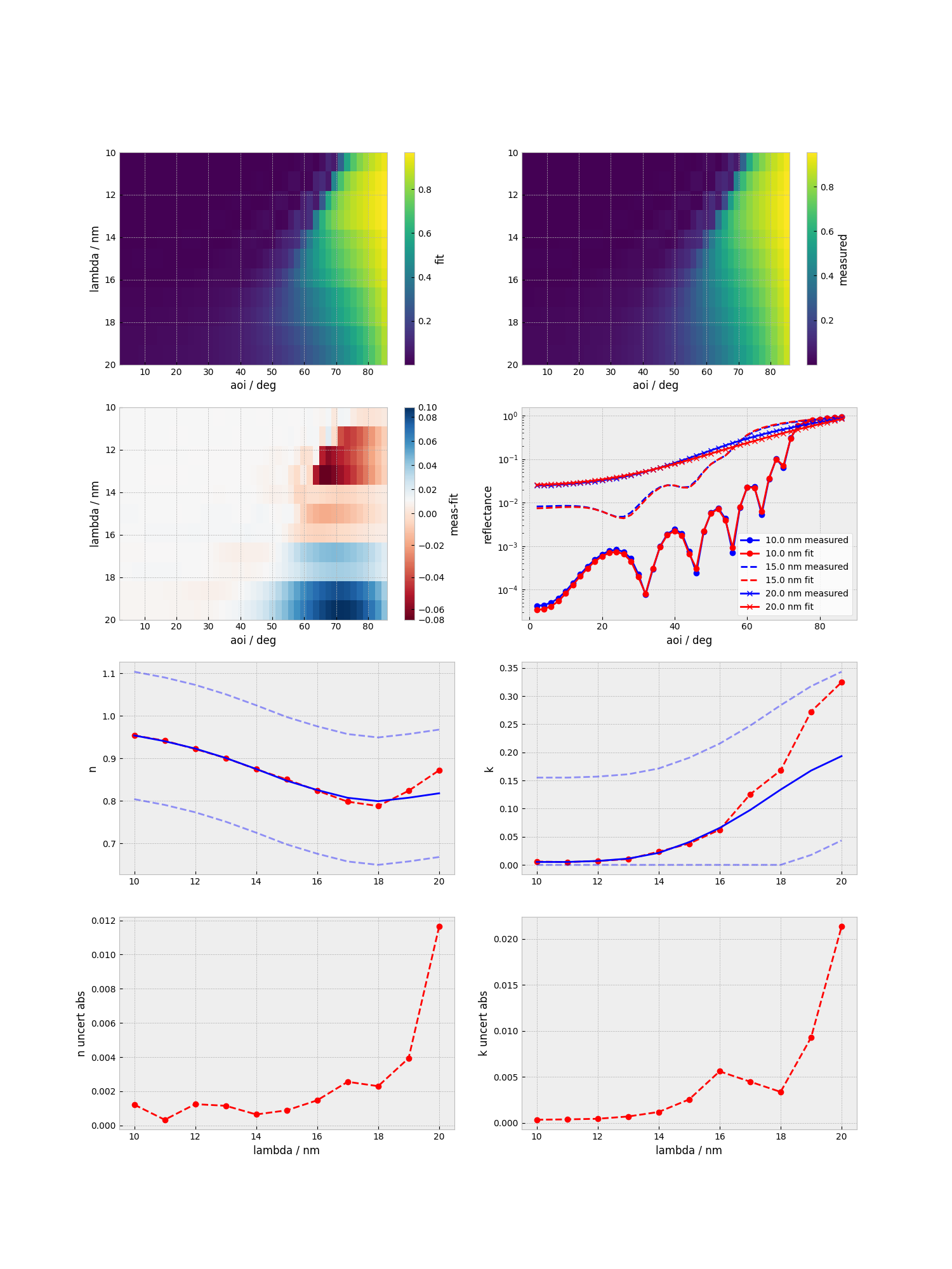
Postprocessing

The MCMC wrapper will generate several output files and perform a few postprocessing steps, such as corner and chain plots, already, which are saved as images.

# Load the required python packages
import numpy as np
import emcee
from matplotlib import pyplot as pp
import parameters as par
import corner
import scipy.stats as st
import seaborn as sb
import pandas as pd
import preprocess_mcmc_oc as ppmc
import parameters as par
from matrixmethod import mm_numba as mm

Next, we will load the saved samples from the MCMC run, stored by chains in the data and reshape the data to a (n_samples, n_dimension) format. Note that this will discard a portion of the samples at the start of the chains to account for burnin.

path_Ru_30_2L = "./tutorials/tutorial_nb_data/results_ru_all_wl.h5"

reader_setup_Ru_30_2L = emcee.backends.HDFBackend(path_Ru_30_2L,read_only=True)
samples_setup_Ru_30_2L = reader_setup_Ru_30_2L.get_chain()

# Reshape to [nsamples, ndim]
burnin = int(samples_setup_Ru_30_2L.shape[0] / par.burnin_factor)
chain_Ru_30_2L = samples_setup_Ru_30_2L[burnin:,:,:].reshape(-1,np.shape(samples_setup_Ru_30_2L)[2])
lb, c, ub = np.percentile(chain_Ru_30_2L        , q=(50-34.1,50,50+34.1),axis = 0)

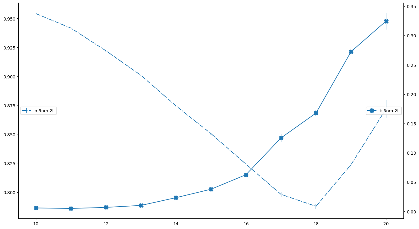
The reconstructed parameters can now be obtain from the sampled posterior distributions by several methods. For example, we can get the median values fot the optical constants and plot them over the wavelengths. Note that when plotting for systems containing more layers, the intervals have to be adjusted accordingly, e.g. c[7:-2:4] instead of c[3:-2:2]. The ordering will always be geometric parameters (thicknesses first, then roughnesses), then optical contants (n and k alternating for each wavelength) and lastly a, then b for the error model.

wl_nm = np.arange(10,21)

fig,ax = pp.subplots()
fig.set_size_inches(16, 9)
fig.set_dpi(val=100)
ax2 = ax.twinx()
ax.errorbar(wl_nm,c[3:-2:2],yerr = (ub-lb)[3:-2:2]/2, label = "n 5nm 2L",color="C0",fmt="-.")

ax2.errorbar(wl_nm,c[4:-2:2],  (ub-lb)[4:-2:2]/2,fmt="-X",color="C0",label ="k 5nm 2L",markersize=10)

# ax2.grid(axis="y")
ax.legend(loc=6)
ax2.legend(loc=5)