Tutorial - Shape Reconstruction via Scatterometry
This tutorial shows how PyThia can be used to approximate the scatterometry measurement process and conduct a global sensitivity analysis of the model.
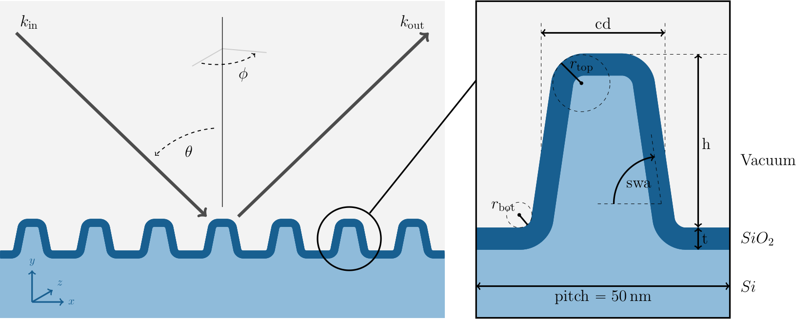
In this experiment a silicon line grating is irradiated by an electromagnetic wave under different angles of incidence \(\theta\) and azimuthal orientations \(\phi\). The aim of this experiment is to build a surrogate for the map from the six shape parameters \(x = (\mathit{h}, \mathit{cd}, \mathit{swa}, \mathit{t}, \mathit{r}_{\mathrm{top}}, \mathit{r}_{\mathrm{bot}})\) to the detected scattered far field of the electromagnetic wave. The experimental setup is visualized in the image below.
Note
If you want to run the source code for this tutorial yourself, you need to download the tutorial data. This tutorial assumes that the data are located in the same directory as the source code.
Surrogate
We start by loading the numpy and pythia packages.
# reshape
angles = np.concatenate([angles, angles], axis=0)  # (180, 2)
Generating training data from the forward problem requires solving Maxwell’s equations with finite elements, which is very intricate and time consuming. We assume the training data we rely on in this tutorial have been previously generated in an “offline” step, on a different machine using the JCMsuite software. Hence we can simply load the data.
y_data = np.concatenate(
    [y_data[:45, :, 0], y_data[:45, :, 1], y_data[45:, :, 0], y_data[45:, :, 1]], axis=0
).T  # (10_000, 180)
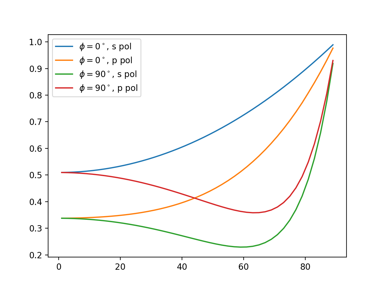
For the simulations we assumed Beta distributed parameters in reasonable parameter domains, which is also the density we drew the samples from. In particular, this implies that the weights are simply \(w_i = 1 / N\), where \(N\) is the number of samples (i.e., \(10.000\) in this case). The scattered intensity signal data consist of 4 curves (2 different azimuthal angles \(\phi\) with s- and p- polarized wave signals each) where each curve is evaluated in 45 points (angles of incidence \(\theta\)). The continuous curves look similar to the image below.
As a first step to compute a polynomial chaos expansion, we need to define the parameters using PyThias Parameter class.
We can use the parameter.npy file to access the parameter information.
            domain=dct["_dom"].tolist(),
            distribution=dct["_dist"],
            alpha=dct["_alpha"],
            beta=dct["_beta"],
        )
    )

print("parameter info:")
print("    parameter  dist    domain    alpha   beta")
print("    " + "-" * 42)
for param in params:
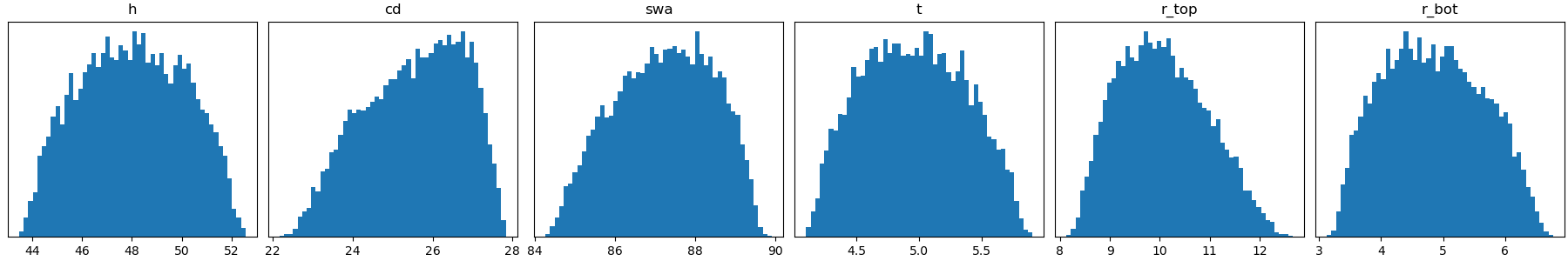
Below you can find a table and an image listing the relevant parameter information.
# |
Name |
distribution |
\(\alpha\) |
\(\beta\) |
|---|---|---|---|---|
1 |
\(\mathit{h}\) |
\(\mathrm{Beta}_{\alpha,\beta}([43, 53])\) |
\(10.0\) |
\(9.67\) |
2 |
\(\mathit{cd}\) |
\(\mathrm{Beta}_{\alpha,\beta}([22, 28])\) |
\(10.0\) |
\(7.76\) |
3 |
\(\mathit{swa}\) |
\(\mathrm{Beta}_{\alpha,\beta}([84, 90])\) |
\(10.0\) |
\(10.13\) |
4 |
\(\mathit{t}\) |
\(\mathrm{Beta}_{\alpha,\beta}([4, 6])\) |
\(10.0\) |
\(11.29\) |
5 |
\(\mathit{r}_{\mathrm{top}}\) |
\(\mathrm{Beta}_{\alpha,\beta}([8, 13])\) |
\(10.0\) |
\(11.10\) |
6 |
\(\mathit{r}_{\mathrm{bot}}\) |
\(\mathrm{Beta}_{\alpha,\beta}([3, 7])\) |
\(10.0\) |
\(12.35\) |
Next, we split the available data into a training and a test set, using roughly \(8.000\) data points for the training.
y_train = y_data[:split]
w_train = w_data[:split]

# test data
x_test = x_data[split:]
y_test = y_data[split:]

# define multiindex set
indices = pt.index.simplex_set(dimension=len(params), maximum=4)
index_set = pt.index.IndexSet(indices)
Now that we have our parameters defined and the training data in place, we only need to define which expansion terms we want to include into our expansion. In this case, we choose a simplex index set to bound the total polynomial degree of the expansion by four. This leaves us with \(210\) polynomial chaos terms in our expansion.
print(f"    dimension: {index_set.shape[1]}")
print(f"    maximum dimension: {index_set.max}")
Finally, we have all the ingredients to compute our polynomial chaos surrogate, which requires only one line of code.
err_abs = np.sum(np.linalg.norm(y_test - y_approx, axis=1)) / y_test.shape[0]
Evaluating the surrogate on our test set with
print(f" L2-L2 error: {err_abs:4.2e} (abs), {err_rel:4.2e} (rel)")
allows us compute an empirical approximation of the \(L^2\)-error (MSE), which is approximately at \(5*10^{-3}\). This is ok, since the measurement error of the observation we will investigate for the inverse problem will be at least one order of magnitude larger.
Sensitivity analysis
There are essentially two different types of sensitivity analyses, local and global.
Local sensitivity analysis typicalls considers a change in the signal by a small variation in the input around a specific point.
Given the polynomial chaos surrogate, computation of the local sensitivities is of course very easy as derivatives of the polynomial are given analytically.
To compute the local sensitivities of the second parameter (\(\mathit{cd}\)) in all points of our test set, i.e. \(\partial/\partial x_{\mathit{cd}}\ f(x_{\mathrm{test}})\), we can use the optional partial argument of the eval() function
local_sensitivity = surrogate.eval(x_test, partial=[0, 1, 0, 0, 0, 0])
However, computing local sensitivities yields only a very limited image of the signal dependency on change in the individual parameter or combinations thereof.
When it comes to estimating whether the reconstruction of the hidden parameters will be possible it is often more reliable to consider the overall dependence of the signal on the parameters.
There are various types of global sensitivity analysis methods, but essentially all of them rely on integrating the target function over the high-dimensional parameter space, which is typically not feasible.
The polynomial chaos expansion, however, is closely connected to the so called Sobol indices, which allows us to compute these indices by squaring and summing different subsets of our expansion coefficients.
The Sobol coefficients are automatically computed with the polynomial chaos approximation and can be accessed via the surrogate.sobol attribute, which is ordered according to the list of Sobol tuples in index_set.sobol_tuples.
As the signal data consist of multiple points on different curves, we get the Sobol indices for each point of our signal.
As this is hard to visualize however, we can have a look on the maximal value each Sobol index takes over the signal points.
The 10 most significant Sobol indices are listed in the table below.
# |
Sobol tuple |
Parameter combinations |
Sobol index value (max) |
|---|---|---|---|
1 |
\((2,)\) |
\((\mathit{cd},)\) |
\(0.9853\) |
2 |
\((4,)\) |
\((\mathit{t},)\) |
\(0.8082\) |
3 |
\((1,)\) |
\((\mathit{h},)\) |
\(0.3906\) |
4 |
\((3,)\) |
\((\mathit{swa},)\) |
\(0.2462\) |
5 |
\((2, 5)\) |
\((\mathit{cd}, \mathit{r}_{\mathrm{top}})\) |
\(0.0332\) |
6 |
\((5,)\) |
\((\mathit{r}_{\mathrm{top}},)\) |
\(0.0240\) |
7 |
\((3, 5)\) |
\((\mathit{swa}, \mathit{r}_{\mathrm{top}})\) |
\(0.0137\) |
8 |
\((1, 2)\) |
\((\mathit{h}, \mathit{cd})\) |
\(0.0065\) |
9 |
\((6,)\) |
\((\mathit{r}_{\mathrm{bot}},)\) |
\(0.0059\) |
10 |
\((2, 3, 5)\) |
\((\mathit{cd}, \mathit{swa}, \mathit{r}_{\mathrm{top}})\) |
\(0.0030\) |
We see that all single parameter Sobol indices are among the top ten, implying that changes in single parameters are among the most influential. Moreover, looking at the actual (maximal) values, we can assume that the first 4 parameters (\(\mathit{h}\), \(\mathit{cd}\), \(\mathit{swa}\), \(\mathit{t}\)) can be reconstructed very well, whereas the sensitivities of the corner roundings \(\mathit{r}_{\mathrm{top}}\) and \(\mathit{r}_{\mathrm{bot}}\) imply that we will get large uncertainties in the reconstruction.
This concludes the tutorial.
Complete Script
The complete source code listed below is located in the tutorials/ subdirectory of the repository root.
  1"""Tutorial - Shape Reconstruction via Scatterometry."""
  2
  3import numpy as np
  4import pythia as pt
  5
  6angles = np.load("angles.npy")  # (90, 2)
  7
  8# reshape
  9angles = np.concatenate([angles, angles], axis=0)  # (180, 2)
 10angle_idxs = [range(45), range(45, 90), range(90, 135), range(135, 180)]
 11angle_labels = [
 12    "$\\phi=0^\\circ$, s pol",
 13    "$\\phi=0^\\circ$, p pol",
 14    "$\\phi=90^\\circ$, s pol",
 15    "$\\phi=90^\\circ$, p pol",
 16]
 17print("angle info:")
 18print(f"    azimuth phi: {np.unique(angles[:,0])}")
 19print(f"    incidence theta: {np.unique(angles[:,1])}")
 20
 21# load data
 22x_data = np.load("x_train.npy")  # (10_000, 6)
 23y_data = np.load("y_train.npy")  # (90, 10_000, 2)
 24w_data = np.load("w_train.npy")  # (10_000, )
 25
 26# reshape y_data
 27y_data = np.concatenate(
 28    [y_data[:45, :, 0], y_data[:45, :, 1], y_data[45:, :, 0], y_data[45:, :, 1]], axis=0
 29).T  # (10_000, 180)
 30print("data info:")
 31print(f"    x_data.shape: {x_data.shape}")
 32print(f"    w_data.shape: {w_data.shape}")
 33print(f"    y_data.shape: {y_data.shape}")
 34
 35# load parameters
 36params = []
 37for dct in np.load("parameter.npy", allow_pickle=True):
 38    params.append(
 39        pt.parameter.Parameter(
 40            name=dct["_name"],
 41            domain=dct["_dom"].tolist(),
 42            distribution=dct["_dist"],
 43            alpha=dct["_alpha"],
 44            beta=dct["_beta"],
 45        )
 46    )
 47
 48print("parameter info:")
 49print("    parameter  dist    domain    alpha   beta")
 50print("    " + "-" * 42)
 51for param in params:
 52    print(
 53        f"    {param.name:<8}  ",
 54        f"{param.distribution:<5}  ",
 55        f"{str(np.array(param.domain, dtype=int)):<7}  ",
 56        f"{param.alpha:<4.2f}  ",
 57        f"{param.beta:<4.2f}",
 58    )
 59
 60# split training/test dataset
 61split = int(0.8 * x_data.shape[0])
 62
 63# training data
 64x_train = x_data[:split]
 65y_train = y_data[:split]
 66w_train = w_data[:split]
 67
 68# test data
 69x_test = x_data[split:]
 70y_test = y_data[split:]
 71
 72# define multiindex set
 73indices = pt.index.simplex_set(dimension=len(params), maximum=4)
 74index_set = pt.index.IndexSet(indices)
 75
 76print("Multiindex information:")
 77print(f"    number of indices: {index_set.shape[0]}")
 78print(f"    dimension: {index_set.shape[1]}")
 79print(f"    maximum dimension: {index_set.max}")
 80print(f"    number of sobol indices: {len(index_set.sobol_tuples)}")
 81
 82print("compute PC surrogate")
 83# run pc approximation
 84surrogate = pt.chaos.PolynomialChaos(params, index_set, x_train, w_train, y_train)
 85# test approximation error
 86y_approx = surrogate.eval(x_test)
 87
 88# L2-L2 error
 89err_abs = np.sum(np.linalg.norm(y_test - y_approx, axis=1)) / y_test.shape[0]
 90err_rel = np.sum(np.linalg.norm((y_test - y_approx) / y_test, axis=1)) / y_test.shape[0]
 91print(f"    L2-L2 error: {err_abs:4.2e} (abs), {err_rel:4.2e} (rel)")
 92
 93# C0-L2 error
 94err_abs = np.sum(np.max(np.abs(y_test - y_approx), axis=1)) / y_test.shape[0]
 95err_rel = (
 96    np.sum(np.max(np.abs(y_test - y_approx) / np.abs(y_test), axis=1)) / y_test.shape[0]
 97)
 98print(f"    L2-C0 error: {err_abs:4.2e} (abs), {err_rel:4.2e} (rel)")
 99
100# global sensitivity analysis
101print("maximal Sobol indices:")
102max_vals = np.max(surrogate.sobol, axis=1)
103l2_vals = np.linalg.norm(surrogate.sobol, axis=1)
104sobol_max = [
105    list(reversed([x for _, x in sorted(zip(max_vals, index_set.sobol_tuples))]))
106]
107sobol_L2 = [
108    list(reversed([x for _, x in sorted(zip(l2_vals, index_set.sobol_tuples))]))
109]
110print(f"    {'#':>2}  {'max':<10}  {'L2':<10}")
111print("    " + "-" * 25)
112for j in range(10):
113    print(f"    {j+1:>2}  {str(sobol_max[0][j]):<10}  {str(sobol_L2[0][j]):<10}")